
Survey sample size is the number of completed responses included in your analysis, written as n. It is different from the number of invitations or people on your list. Under the calculator's sampling assumptions, a larger sample narrows the margin of error; it does not remove biased recruitment or poorly worded questions.
Sample size calculator
Nothing is hidden behind a signup and nothing is sent anywhere. The calculator runs in your browser, starts with a worked answer already on screen, and prints the formula and the arithmetic it used so you can check it or reproduce it by hand.
How many responses do I need?
Set your six inputs. The answer, the formula, and the arithmetic all update as you type.
Completed responses you need
370
After the finite population correction.
People to invite
1,234
At a 30 percent response rate.
Sampling fraction
3.7%
Share of the population you need to hear from.
Total, sized per subgroup
370
The arithmetic, step by step
| Margin of error | Completes needed | Invites needed |
|---|
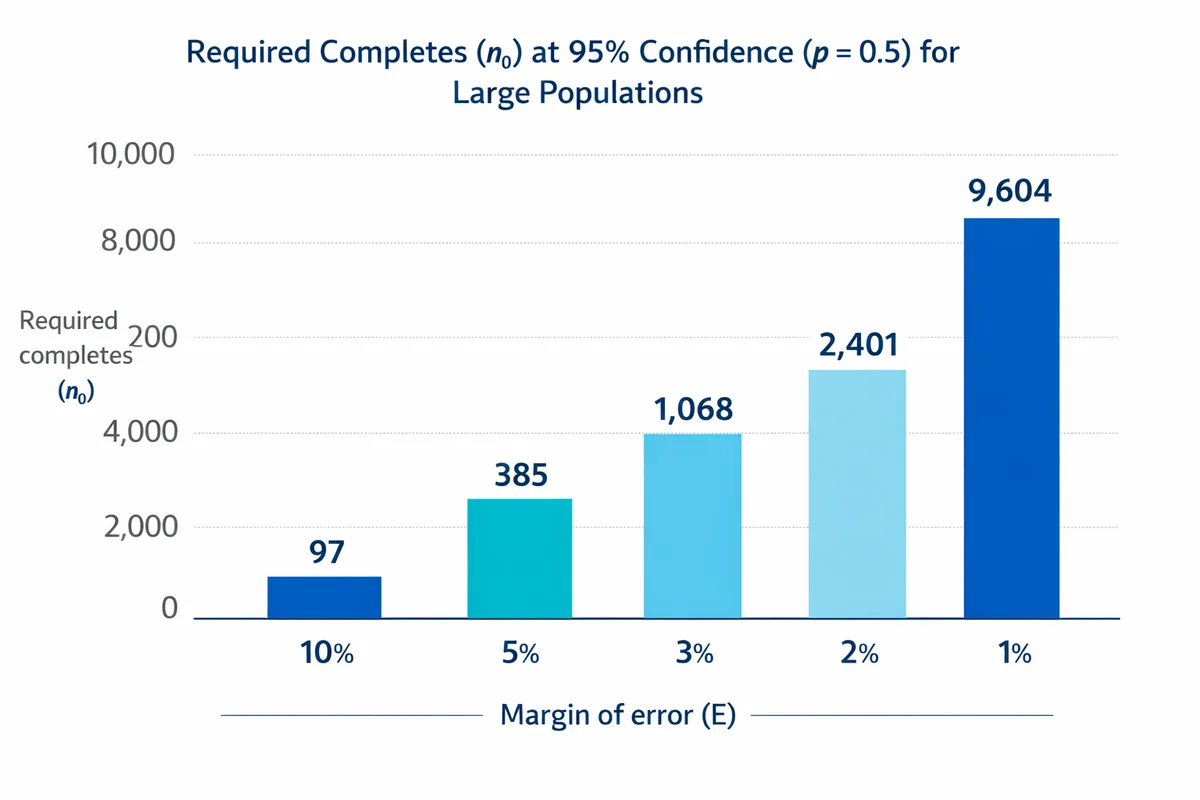
Tighter precision costs responses at roughly the square of the improvement. Halving the margin of error multiplies the sample by about four.
The copy button writes a short methods paragraph with your numbers, the formula, and the citation, ready to paste into a project brief or a methodology chapter.
Cite this calculator: Hodge, M. (2026). Survey Sample Size Calculator. SuperSurvey. https://www.supersurvey.com/Sample-Size
The result is completed responses, not invitations. It is the count you need in hand at the end of fieldwork. The invitation figure is that number divided by the response rate you expect, which is where most sample plans go wrong. Once the target is set, create your survey and pilot it with the intended audience. Use the pilot to check the wording and estimate the invitation-to-completion rate for your own project.
What sample size means
Sample size is the number of people who complete your survey. It is written as n in every formula on this page, it is the one quantity you buy with fieldwork rather than choose on paper, and it is the figure your margin of error is calculated from.
Three counts get mistaken for it, and telling them apart is most of what a sample plan does:
- Population (N): everyone you want to describe. A customer list, a headcount, a country.
- Invitations: how many people you contact. Always larger than n, because not everyone answers.
- Sample size (n): how many completed responses you hold when fieldwork ends. This is the number the formula sizes, and the only one of the three that changes your margin of error.
Sample size buys precision, which is the width of the plus or minus band around each result. It does not buy accuracy, which is whether the people who answered resemble the people who did not. A large convenience sample can sit further from the truth than a small random one, and no value of n repairs that. Where sample size planning goes wrong covers the difference, and how you draw the sample is what decides it.
The short answer, if you only want a number
Key numbers
- 385 completed responses is the default answer. That is what the formula returns at 95 percent confidence, a margin of error of plus or minus 5 percentage points, and no prior estimate of the result.
- Small populations need far fewer. A list of 1,000 people needs 278. A list of 100 needs 80. That is the finite population correction at work.
- Precision is expensive. Halving the margin of error multiplies the sample by about four. Going from plus or minus 5 points to plus or minus 1 point takes you from 385 to 9,604.
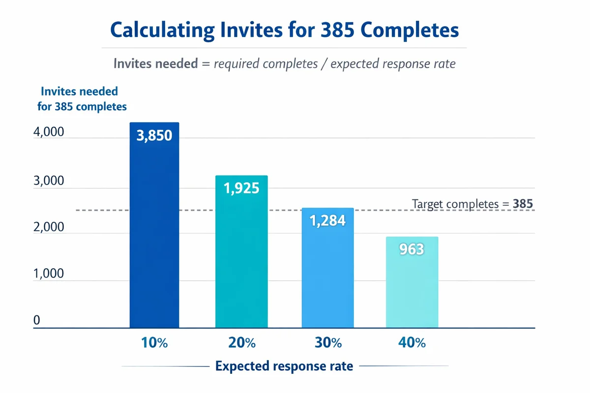
- Formulas count completes, not invites. Invitations needed equals completes divided by your expected response rate. At 30 percent, 385 completes means inviting 1,284 people.
- Margin of error covers one kind of error. It measures the noise from sampling some people instead of all of them. It says nothing about the people who never answered.
The sample size formula, and how to do it by hand
For a survey that reports a percentage, the standard starting point is the sample size for a population large enough to treat as unlimited:
n0 = (z^2 x p x (1 - p)) / E^2
Reading it left to right:
- n0 is the required completed responses, before any population correction.
- z is the z score for your confidence level. Use 1.96 for 95 percent.
- p is the proportion you expect to measure, as a decimal. Use 0.5 if you do not know.
- E is the margin of error as a decimal. Five percentage points is 0.05.
The symbol for sample size is n. Some sources write the uncorrected figure as n0 and the corrected one as n, which is the convention used here.
| Confidence level | z | What it costs you |
|---|---|---|
| 80 percent | 1.282 | 165 completes at plus or minus 5 points |
| 90 percent | 1.645 | 271 completes |
| 95 percent (standard) | 1.960 | 385 completes |
| 99 percent | 2.576 | 664 completes |
| 99.9 percent | 3.291 | 1,084 completes |
Worked example: from 385 to an invitation list
Scenario. You want the percentage of customers who would recommend you. You want 95 percent confidence and plus or minus 5 points. You have no prior estimate, so p = 0.5.
Pick your confidence level and margin of error
95 percent confidence sets z = 1.96. Plus or minus 5 percentage points is E = 0.05.
Choose an expected result
p = 0.5, because there is no prior estimate and 0.5 produces the largest sample. Nothing you learn later can leave you short.
Apply the sample size formula
n0 = (1.96^2 x 0.5 x 0.5) / 0.05^2
n0 = (3.8416 x 0.25) / 0.0025 = 0.9604 / 0.0025 = 384.16
Round up: 385 completed responses. Always round up. You cannot collect a fraction of a survey.
Correct for a small population
If those customers are a list of 1,000 rather than an open market, apply the correction: n = 384.16 / (1 + 383.16 / 1,000) = 384.16 / 1.38316 = 277.7, so 278 completes. The correction only bites once the sample is a large share of the population.
Turn completes into invitations
At a 30 percent response rate, invitations = 278 / 0.30 = 926.7, so invite 927 people. Completes are what the formula sizes. Invitations are what you actually send, and they can never exceed the population you are drawing from.
At 95 percent confidence with p = 0.5, the whole formula collapses to 0.9604 divided by E squared. That single shortcut answers most sample size questions in one line, and it is why 385 keeps appearing in sample size tables you find elsewhere.
Sample size table for common population sizes
These figures are computed with the formula above at 95 percent confidence, plus or minus 5 points and p = 0.5, then corrected for the population. The last two columns are our own check against the table published by Krejcie and Morgan in 1970, which is the table most methods chapters cite.
| Population (N) | Completes needed | Krejcie and Morgan (1970) | Difference |
|---|---|---|---|
| 10 | 10 | 10 | same |
| 25 | 24 | not listed | |
| 50 | 45 | 44 | 1 more |
| 100 | 80 | 80 | same |
| 200 | 132 | 132 | same |
| 500 | 218 | 217 | 1 more |
| 1,000 | 278 | 278 | same |
| 2,000 | 323 | 322 | 1 more |
| 5,000 | 357 | 357 | same |
| 10,000 | 370 | 370 | same |
| 50,000 | 382 | 381 | 1 more |
| 100,000 | 383 | 384 | 1 fewer |
How we checked it. We ran the formula at 21 population sizes and compared each result with the published Krejcie and Morgan value. Twelve matched exactly. The other nine differed by exactly one response, which comes from where each method rounds, not from a disagreement about the arithmetic. If a supervisor asks why your number differs from the table by one, that is the reason.
Worth knowing if you are citing that table: Krejcie and Morgan did not derive their own formula. Their 1970 paper is about 400 words plus one table, and its single reference credits the formula to a 1960 research bulletin from the National Education Association. Their own summary of the pattern is still the best one line description of it, that as the population grows the required sample increases at a diminishing rate and settles at slightly more than 380 cases.
Choosing your inputs, one at a time
Four numbers drive the answer. Three of them are decisions, not facts, and each one has a defensible way to pick it.
Confidence level: how often the method is right
Confidence level describes the method, not this particular survey. At 95 percent confidence, intervals built this way contain the true value 95 times out of 100 in the long run. It is not a 95 percent chance that your specific answer is correct.
Use 95 percent unless you have a reason not to. Moving to 99 percent raises the sample from 385 to 664 for the same precision, which is a 72 percent cost increase to buy very little. The related idea in hypothesis testing is alpha, which is why people mix the two up. If that distinction is fuzzy, read statistical significance and what p-values mean before you pick a number.
Margin of error: the decision variable
This is the one to think hardest about, because it is the only input that ties the sample to a decision. Pick it by asking what gap would change what you do.
If you act differently when satisfaction is 72 percent rather than 74 percent, you need a tight margin. If you only act at 72 versus 82, plus or minus 5 points is plenty. Broad top-line reporting usually lands at 5 points for a pulse check or 3 points for tracking. Below 2 points the cost climbs fast.
Population size: mostly irrelevant, until it is not
For big populations the required sample barely moves. Ten thousand people need 370 responses. A hundred thousand need 383. Population size only bites when your sample is a meaningful share of it, which is the case for employee lists, member registers and school cohorts. That is what the next section handles.
Expected result (p): use 0.5 when you do not know
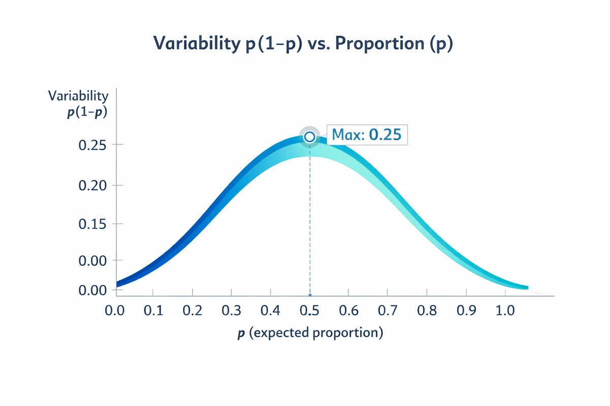
For a percentage question, the uncertainty is driven by p times (1 minus p). That term is largest at p = 0.5, so 0.5 is the conservative choice and produces the largest sample. It is the right default when you have no prior estimate.
If you do have one, use it, because the saving is large. At 95 percent confidence and plus or minus 5 points, p = 0.5 asks for 385 responses and p = 0.9 asks for 139. Past surveys, a pilot, or a published benchmark are all fair sources for that estimate. Noisy questions inflate the spread too, so clearer wording can stabilise a result without any extra responses. Writing better survey questions is often cheaper than collecting more of them.
Small populations: the finite population correction
The base formula assumes you are drawing from a pool deep enough that removing people from it changes nothing. Once your sample is a real slice of the population, that assumption overcharges you. The finite population correction gives the responses back.
n = n0 / (1 + ((n0 - 1) / N))
- n is the corrected number of completes you need.
- n0 is the uncorrected figure from the formula above.
- N is the population size.
The usual trigger is that n0 is more than about 5 percent of N. Below that the correction changes almost nothing, so it is not worth explaining to anyone.
Worked example: an employee survey
Scenario. You have 1,200 employees. You want 95 percent confidence, plus or minus 5 points, and you use p = 0.5.
- Uncorrected, n0 = 384.16.
- Corrected: n = 384.16 / (1 + (383.16 / 1,200)) = 384.16 / 1.3193 = 291.2.
- Round up: 292 completed responses.
Without the correction you would chase 385 responses from a list of 1,200, which is 32 percent of everyone. With it, 292 buys the same precision. On a list that size that is a month of chasing you do not have to do.
Below roughly 200 people the corrected sample is such a large share of the list that inviting everybody is simpler and more defensible. A census of 150 people has no sampling error at all. Your effort then goes into response rate and into who is missing, which is where it belongs.
Margin of error: the same formula, run backwards
Margin of error is the plus or minus band around a survey result that comes from having asked some people instead of all of them. If 62 percent of 385 respondents pick an option and the margin of error is 5 points, you report 62 percent and say the plausible range runs from 57 to 67 percent.
Rearranging the sample size formula to solve for E gives:
E = z x square root of (p x (1 - p) / n)
With a finite population, multiply that by the square root of (N - n) divided by (N - 1). Both versions are in the calculator below, which switches automatically when you tick or untick the population box.
What is the margin of error on the responses I already have?
The same formula, rearranged. Put in the responses you collected and read the precision back.
Margin of error
5.0
Percentage points, plus or minus.
Your interval
45.0 to 55.0
Percent, at 95 percent confidence.
The arithmetic, step by step
Does margin of error increase with sample size?
It shrinks, and it shrinks with the square root of n. That square root is the whole economics of surveys. Four hundred responses give you half the error of one hundred. To halve it again you need 1,600. Each further decimal place of precision costs roughly four times the fieldwork, which is why 385 is such a common landing point: it is where cost and precision stop arguing.
Four terms people mix up
Standard error, margin of error, confidence level and confidence interval get used as though they were interchangeable. They are four different things, and the difference matters when someone questions your number.
| Term | What it is | At 385 responses and 50 percent |
|---|---|---|
| Standard error | The raw spread of the estimate. The square root of p times (1 minus p) divided by n. | 0.0255, or 2.55 percentage points |
| Margin of error | The standard error multiplied by a z score for the confidence level you chose. | Plus or minus 5.0 points at 95 percent |
| Confidence level | The z score you picked, expressed as a percentage. A choice, not a measurement. | 95 percent, so z = 1.96 |
| Confidence interval | The result with the margin of error applied, written as a range. | 45.0 percent to 55.0 percent |
The short version: standard error is a property of your data, confidence level is a choice you made, margin of error is the two multiplied together, and the confidence interval is what you print in the report.
What the margin of error does not cover
It covers random sampling error and nothing else. It does not cover people who ignored the invitation, a list that was missing part of the population, or a question that half your respondents read differently from the way you meant it. A survey can have a tidy margin of error and still be wrong. See response bias and nonresponse bias for the errors that no sample size fixes.
The professional body for survey research puts this more bluntly than most vendors will. AAPOR states that there is no such thing as a measurable overall margin of error for a poll, because surveys carry other errors that cannot be measured at all, from how the questions were written to how the interviews were run. What you can compute is the sampling piece. That is the piece the calculator gives you, and it is worth being clear that it is a piece.
Two usage rules from the same source, both of which most survey writing gets wrong:
- It is percentage points, not a percentage. Write "plus or minus 3 percentage points", not "plus or minus 3 percent". They mean different things.
- It does not apply to opt-in samples at all. A margin of error assumes every person had a known, non-zero chance of selection. An open link, a panel of volunteers or a social media post does not meet that. Publishing a margin of error next to results from an open link is claiming a precision you did not buy.
Turning completes into invitations
The formula gives you finished responses. Fieldwork gives you a response rate. The gap between them is where sample plans usually fail, and the arithmetic is one line:
Invitations = required completes / expected response rate
Use the rate as a decimal, so 30 percent is 0.30, and round up. For 292 completes at 35 percent, that is 292 divided by 0.35 = 834.3, so invite at least 835 people.
| Completes needed | Expected response rate | Invitations |
|---|---|---|
| 385 | 60 percent | 642 |
| 385 | 30 percent | 1,284 |
| 385 | 15 percent | 2,567 |
| 292 | 50 percent | 584 |
| 292 | 35 percent | 835 |
| 292 | 20 percent | 1,460 |
Picking a response rate you can defend
Your own history beats any published benchmark, as long as it is the same audience, the same channel and a similar length of survey. If you have nothing to go on, plan three scenarios at 20, 30 and 40 percent and treat the invitation list as an adjustable lever during fieldwork. Reminders, a longer window and a wider list are all things you can change midway. The completes target is not.
Most benchmark tables on the internet quote one average with no source. There is no single average. Here is what the primary sources actually report, so you can cite the row that matches your situation instead of a number somebody made up.
| Setting | Response rate | Scale and source |
|---|---|---|
| US federal agencies under 1,000 staff | 71 percent | 2024 Federal Employee Viewpoint Survey (OPM) |
| US federal agencies of 1,000 to 9,999 staff | 60 percent | Same survey, same year (OPM) |
| US federal agencies over 75,000 staff | 37 percent | Same survey, same year (OPM) |
| All US federal employees | 41 percent | Over 1.6 million invited, over 674,000 responded, 2024 (OPM) |
| Published online surveys, all kinds | 44.1 percent mean | Meta-analysis of 1,071 reported rates (Wu and colleagues, 2022) |
| Published organisational research | 68 percent in 2020, up from 48 percent in 2005 | 1,014 surveys across 17 journals (Holtom and colleagues, 2022) |
| Telephone polling of the general public | 6 percent in 2018, down from 36 percent in 1997 | Pew Research Center's own tracked rate (Kennedy and Hartig, 2019) |
| Web mode versus any other mode | about 12 points lower | Meta-analysis of 114 experimental comparisons (Daikeler and colleagues, 2020) |
Two things fall out of that table. First, the size of the group you are surveying predicts the rate better than almost anything else you control. A 300 person company and a 300,000 person agency are not running the same survey. Second, the widely repeated claim that response rates are collapsing everywhere is only true in some places. Telephone polling did collapse. Published organisational research went the other way, from 48 percent to 68 percent over fifteen years.
One more piece of planning arithmetic worth borrowing: the standard extension guidance is to add about 10 percent to your invitation list for people you simply cannot reach, and about 30 percent for people who could answer and do not.
What our own template corpus says about length
A response rate borrowed from someone else's survey travels badly, and length is one of the few things on that list you fully control. Here is a figure we can produce and a competitor cannot, because it comes from counting our own published corpus rather than asking practitioners what they think they do.
In our 21 August 2026 audit, all 87 survey templates were 14 questions or shorter, and 86 were 10 questions or shorter. Together they held 799 questions. The median was 9 questions and exactly one template ran past 10. These figures describe that dated snapshot, not the current library.
| Questions in the template | Templates | Share of the corpus |
|---|---|---|
| 7 questions | 4 | 5 percent |
| 8 questions | 17 | 20 percent |
| 9 questions | 29 | 33 percent |
| 10 questions | 36 | 41 percent |
| 14 questions | 1 | 1 percent |
By answer format, 355 of the 799 questions are rating scales, 281 are single choice lists, and 163 ask the reader to type something. That last group is the one that costs you completions, so we read it by hand instead of trusting the stored field. Of the 163, 137 are multi line comment boxes. The other 26 are single line boxes, and reading them showed that 22 are short identifier or classification fields: a name, an email address, a date, a department, a job title. Only 4 are substantive short answers. So the honest count of genuinely open ended questions is 141, or roughly one question in six, not the one in five the raw field would have handed us.
How we counted, and how we checked it. We parsed the stored question list of every survey template live on this site on 21 August 2026, kept the entries carrying question text, then fetched each published page and compared the two sets rather than trusting our own database on its own. All 87 pages returned HTTP 200, while a slug we know is dead returned 410 in the same run, so the check was discriminating rather than uniformly green. 785 of the 799 questions, or 98 percent, appear on the published page. Six of those matches differ from the database only in which apostrophe character is used, and we counted them as matches, which we would rather disclose than quietly round away. Eighty six of the 87 templates verified in full. The one that did not is our longest, at 14 questions, and its published page currently renders no preview questions at all, so its questions could not be confirmed from the outside.
Template length does not tell you the invitation response rate. Our separate survey response benchmark examines behavior after people interact with a survey; it does not count everyone invited. For invitation planning, use a documented rate from a comparable project or a pilot, and keep the denominator consistent.
The practical use is narrow and real. If you are borrowing a response rate for the invitation count in the calculator, borrow it from a survey about the length of the one you are about to send, to a similar audience on a similar channel. Our own published instruments sit between 7 and 10 questions, which is shorter than most drafts start out.
More invitations do not buy you less bias
A low response rate creates two problems that look like one. The first is that you finish short of your target, so your margin of error is wider than you planned. The second is that the people who answered may differ from the people who did not, in ways that matter to your result.
Inviting more people fixes the first problem. It does not reliably fix the second. Groves and Peytcheva pooled 59 studies that measured actual nonresponse bias against known truth, and found only a small relationship between a survey's response rate and how biased it turned out to be. Pew tested the same idea directly: they ran one questionnaire twice, once with standard methods that got a 9 percent response rate and once with a high effort protocol that got 22 percent. Of the 40 questions the two surveys shared, 28 came back within 2 points of each other.
The honest counter-case. That finding does not generalise to every topic, and it is worth knowing where it breaks. In satisfaction surveys the relationship is real and large. A study of 717 hospital patient satisfaction surveys across 164 Swiss hospitals found mean satisfaction score and response rate correlated at r = 0.61, because delighted and furious people answer and the ambivalent middle does not. If you run CSAT or NPS, a rising response rate can move your score on its own, and a low one probably flatters you.
So: chase response rate when you are measuring how people feel about you. Do not treat it as a certificate of validity when you are measuring anything else.
Sample size for quantitative research: what a methods chapter needs
There is no single good sample size for quantitative research, and any source that gives you one without asking what you are measuring is guessing. What gets a methods chapter approved is not a large number. It is a stated number, with the confidence level, margin of error, assumed proportion and population written next to it, and a named formula attached.
Supervisors tend to expect one of four named approaches. They mostly agree with each other, and it is worth knowing which one you are being asked for.
| Named approach | What it asks you for | Result for N = 1,000 at 95 percent and 5 points | Use it when |
|---|---|---|---|
| Cochran (1977) | z, p, E, then the finite population correction if the population is small | 278 | The default. It is the formula on this page, and the one the others are derived from. |
| Krejcie and Morgan (1970) | Nothing. You read the answer off a published table by population size. | 278 | You want a citable table rather than arithmetic. It is Cochran at fixed settings. |
| Yamane (1967), often called Slovin | Only N and the margin of error | 286 | Only when p really is unknown and you accept 95 percent confidence baked in. See the caution below. |
| Power analysis | Effect size, power, alpha and the test you will run | Depends entirely on the effect size | You are testing a hypothesis rather than estimating a percentage. Use G*Power or OpenEpi, not this page. |
Cochran, and why everything else is a shortcut of it
Cochran's formula is the one at the top of this page: n0 = z squared times p times (1 minus p), divided by E squared, followed by the finite population correction when the population is small. The other named methods fix some of those inputs to make the arithmetic shorter. Once you know that, the family stops looking like four competing rules and starts looking like one rule with three presets.
Yamane and Slovin: use with your eyes open
The formula n = N / (1 + N x e^2) appears in thousands of theses, usually credited to Slovin. It is quick: for N = 1,000 and e = 0.05 it gives 286.
Three things are worth knowing before you cite it.
- It is Cochran with the settings welded shut. Working backwards, the formula is the proportion formula with p fixed at 0.5, confidence fixed at 95 percent, and z rounded from 1.96 to 2. It cannot answer a question at any other confidence level, and it has no input at all for how variable your population is. Two populations of the same size but wildly different spread get the same answer, which cannot be right.
- That rounding is why its numbers run high. With z = 2 the formula's ceiling for an unlimited population is exactly 1 divided by e squared, which is 400. Cochran's ceiling is 384.16, because 1.96 squared is 3.8416 and not 4. Every Yamane figure in the table above is a few percent larger than the Cochran figure for exactly that reason. If you have ever wondered why two textbooks give you two different sample sizes for the same study, that is usually the answer.
- The attribution does not hold up. A statistics journal traced the formula's history and concluded that no person named Slovin can be found behind it, and that the oldest traceable source is Taro Yamane's 1967 textbook. Wolfram MathWorld describes it as an ad hoc formula lacking mathematical rigour. If your department expects it, use it and cite Yamane rather than Slovin. If you have a choice, use Cochran, because it survives the question of where the 95 percent came from.
Rules of thumb, honestly graded
These circulate widely. Some are useful, some are folklore, and it helps to know which is which.
- At least 30 per group. Reasonable as a floor for group comparisons, not as a target. It comes from where sampling distributions start behaving, not from any precision requirement.
- Ten cases per variable in a regression. A working heuristic, widely used and widely criticised. State it as a heuristic, never as a rule.
- Ten percent of the population. This one is simply wrong and the table above shows why. Ten percent of 100,000 is 10,000 responses, when 383 gives you the same precision.
- Always 385. Right only for a large population at 95 percent and 5 points. Quote it with those conditions attached or it means nothing.
- Small n for usability and product studies. Nielsen Norman Group publishes the honest version of this: 40 participants gets you a yes or no measure to plus or minus 15 points at 95 percent confidence, and 47 gets you an average to the same precision. Those numbers are small because the precision claimed is loose. Say the precision out loud and small samples stop being embarrassing.
If your study compares groups rather than estimating one percentage, sample size becomes a power question and this is not the right calculator. You need an effect size you are willing to defend, plus alpha and power. G*Power and OpenEpi are the free tools most supervisors expect, and both are free. Saying where a tool stops is more useful than pretending it does everything.
Qualitative work is sized differently
Interviews and focus groups are not sized with a margin of error, because they are not estimating a population percentage. The usual argument is saturation: you keep going until new participants stop producing new themes, then report where that happened and how you judged it. Running a qualitative study through this calculator produces a number that looks precise and means nothing.
If you need results by subgroup, size for the subgroup
Most surveys are asked to report by region, role, tenure or product line. This is where sample plans quietly break, and the rule is short.
Your margin of error applies to a group only if that group has that many completes. If you want plus or minus 5 points for each of six regions, you need roughly 385 completes in each region, not 385 in total. That is a survey six times the size you thought you were planning.
Two honest ways out:
- Oversample the small groups. Deliberately invite a higher share of the smaller segments so each one reaches its own target. You weight the results back afterwards.
- Accept wider bands for the breakouts. Keep one strong overall number and publish each subgroup with its own, larger margin of error next to it. This is usually the right answer.
The calculator has a field for this. Set Subgroups to report separately to the number of groups you owe a result for, and it sizes each group properly and totals them.
Scope it before you field. List the segments you must report, not the ones that would be nice to have. Estimate the completes each one can realistically produce, using demographic questions to identify them. If a segment can only yield 80 responses, do not promise plus or minus 5 points for it. At 80 responses the band is plus or minus 11 points.
AAPOR uses a worked example that is worth memorising. A survey of 1,000 adults carries an overall margin of error of about plus or minus 3 points. If 200 of those people are the subgroup you actually want to talk about, that subgroup's margin of error is plus or minus 6.9 points, more than double. The headline figure on the front of the report is not the figure that governs the chart on page nine.
Published guidance on minimum cell sizes is older and looser than the formulas, and it is fair to treat it as a floor rather than a target: roughly 100 responses for a subgroup you will report on properly, and 20 to 50 for a minor one you will mention in passing.
Where sample size planning goes wrong
Sample size manages sampling error, the random noise from not asking everyone. Real surveys also carry systematic error, which no sample size fixes and which a large sample can disguise.
Treating a convenience sample like a probability sample
Every formula here assumes each person had a known, non-zero chance of being selected, and that answering was not strongly tied to what you are measuring. An open link on social media meets neither condition. You can still compute a margin of error from the responses, and it will look reassuring, and it will not mean what it says. Be explicit about which kind of sample you actually drew.
Reading a bigger n as better measurement
A large sample makes a noisy measurement precisely noisy. If a question is ambiguous, double-barrelled or leading, more responses will not rescue it. High skip rates and inconsistent answers are signs to fix the instrument first. Rewriting one bad question often does more than tripling the sample.
Choosing precision without a decision behind it
Precision only has a right answer once you know what it is for. A sample size is easy to defend when you can finish this sentence: we need to tell apart outcomes that differ by X points. It is impossible to defend when the only rationale is that a bigger number felt safer. Tie it back to your research design and to what you will do with the result.
The numbers on this page, and how good they are
Every figure quoted above is either arithmetic you can reproduce in the calculator or a citation you can check. Grade A means replicated or directly computable, B means a single strong study, C means widely repeated but contested.
| Claim | Number | Grade | Source |
|---|---|---|---|
| At 95 percent confidence with no prior estimate, a large population needs 385 completed responses for plus or minus 5 points. | 385 | A | Direct arithmetic from the standard proportion formula. NIST section 3.3.3; Israel (1992). |
| The formula on this page reproduces the published Krejcie and Morgan sample size table to within one response at every one of 21 population sizes we checked. | 21 of 21 within 1 | A | Our own check against Krejcie and Morgan (1970). Method stated below the table. |
| Response rate is a weak predictor of nonresponse bias. A meta-analysis of 59 dedicated bias studies found only a small relationship between the two. | 59 studies | A | Groves and Peytcheva (2008), Public Opinion Quarterly. |
| Pew ran the same questionnaire at a 9 percent and a 22 percent response rate. Of 40 shared questions, 28 came back within 2 points. | 28 of 40 within 2 points | B | Pew Research Center (2012), Assessing the Representativeness of Public Opinion Surveys. |
| But in satisfaction surveys the relationship is real and large. Across 717 hospital surveys, mean satisfaction score correlated with response rate at r = 0.61. | r = 0.61 | B | Perneger, Peytremann-Bridevaux and Combescure (2020), BMC Health Services Research. |
| Employee survey response rate tracks organisation size almost perfectly. In 2024 the US federal employee survey got 71 percent from agencies under 1,000 people and 37 percent from agencies over 75,000. | 71 vs 37 percent | A | US Office of Personnel Management (2024), FEVS Governmentwide Management Report, over 1.6 million employees invited. |
| The mean response rate across 1,071 published online surveys was 44.1 percent. There is no single normal rate. | 44.1 percent | A | Wu, Zhao and Fils-Aime (2022) meta-analysis, Computers in Human Behavior Reports. |
| Web surveys return about 12 percentage points lower response than other modes, across 114 experimental comparisons. | 12 points lower | A | Daikeler, Bosnjak and Lozar Manfreda (2020) meta-analysis, JSSAM. |
| Halving the margin of error multiplies the required sample by about four, because n scales with 1 over E squared. Doubling a sample from 1,000 to 2,000 buys about one point. | about 4x | A | Algebraic property of the formula; AAPOR states the 1,000 to 2,000 case explicitly. |
| Assuming p = 0.5 instead of a known p = 0.9 nearly triples the sample you are told to collect, from 139 to 385. | 139 vs 385 | A | Direct arithmetic. Reproducible in the calculator by changing the expected result. |
| All 87 survey templates published on this site are 14 questions or shorter, and 86 of the 87 are 10 or shorter. 785 of their 799 questions were confirmed on the published pages. | 87 templates, 799 questions | A | Our own count of the live template corpus, 21 August 2026, checked back against all 87 published pages. Method, hand audit and verification rate stated with the table. |
| There is no traceable person named Slovin behind the formula that carries the name. The oldest traceable source is Yamane (1967). | no traceable author | B | Tejada and Punzalan (2012), The Philippine Statistician; Wolfram MathWorld calls it ad hoc. |
"You always need 385 responses." Only at 95 percent confidence, plus or minus 5 points, p = 0.5 and a large population. Quoted bare, it is wrong for every small population.
"Survey 10 percent of your population." There is no statistical basis for it. It wildly oversamples big populations and undersamples small ones.
"A response rate below 50 or 60 percent invalidates a survey." No threshold does that. The 50, 60 and 70 percent ladder is a textbook rule of thumb with no empirical derivation behind it, and the Groves and Peytcheva meta-analysis contradicts it. Response rate bounds the worst case bias. It does not measure the actual bias.
"The average survey response rate is X percent." Verified figures from the same few years run from 6 percent to 71 percent depending entirely on who is being surveyed. Any single average is hiding that. Cite the row that matches your situation from the table above instead.
Slovin's formula presented as a derivation. It is Cochran's formula with 95 percent confidence and p = 0.5 baked in and z rounded to 2, and the Slovin attribution has no traceable source.
The justification template
Most sample size arguments fail because the assumptions were never written down. The Copy the justification button in the calculator writes this out with your own numbers already in it. If you would rather assemble it yourself, these are the nine things a reviewer will look for.
- Population (N): define the population and state the count. For example, all active customers in the last 90 days, N = 48,200.
- What you are measuring: a proportion (a percentage) or a mean (an average rating). The formula here sizes proportions, which covers most reported KPIs.
- Confidence level: the level you chose and why. Convention and risk tolerance are both acceptable reasons if you say so.
- Margin of error (E): your target precision overall, and separately for any subgroup you promised to report.
- Assumed proportion (p): the value used, and where it came from. State plainly if it is 0.5 because nothing better was available.
- Finite population correction: whether you applied it and what triggered it, such as n0 exceeding 10 percent of N.
- Completes target (n): the final required number of completed responses after every adjustment.
- Expected response rate: the rate assumed, the history it came from, and the resulting invitation count.
- How you will select people: simple random, stratified, census, or convenience, plus any oversampling for key segments. Name it honestly.
Once the survey is in the field, keep watching completes by segment rather than the total. A healthy overall number can hide a segment that will never reach its target, and that is a problem you can still fix at week one and cannot fix at week four. When you report, pair every percentage with its margin of error, and read how to analyse survey data before treating a two point move as real.
Sample size planning worksheet
One page you can print, fill in by hand, and staple to a project brief. Fill the middle column before fieldwork starts, not after. Nothing is sent anywhere and no account is needed.
| Decision | Your value | Prompt |
|---|---|---|
| Population (N) | Who exactly, and how many of them. Write the definition, not just the number. | |
| What you are measuring | A percentage or an average. This page sizes percentages. | |
| Confidence level | 95 percent unless you have a reason. Write the reason. | |
| Margin of error (E) | The gap you need to be able to tell apart, in points. | |
| Assumed proportion (p) | 0.5 if nothing better exists. Say where a different value came from. | |
| Finite population correction | Applied or not, and what triggered it. | |
| Completes target (n) | The final figure after every adjustment. | |
| Subgroups reported separately | How many, and the completes each one owes on its own. | |
| Expected response rate | The rate, and the history behind it. Not a number off the internet. | |
| Invitations to send | Completes divided by the rate, rounded up. Never more than N. | |
| How people are selected | Random, stratified, census or convenience. Name it honestly. | |
| Fieldwork checkpoint | The date you will check completes by segment, not just the total. |
Formula: n0 = (z^2 x p x (1 - p)) / E^2, then n = n0 / (1 + (n0 - 1) / N). Source: Cochran (1977); NIST/SEMATECH e-Handbook section 3.3.3; Israel (1992). Worksheet from https://www.supersurvey.com/Sample-Size
Frequently Asked Questions
What is sample size?
Sample size is the number of completed responses in a survey, written as n. It is not the number of people you invited, and it is not the size of the population you are describing. It is the count you finish fieldwork with, and it is the figure your margin of error is computed from: 385 completed responses gives about plus or minus 5 points at 95 percent confidence when the population is large. What sample size means sets out the difference between the population, the invitations and n.
How many responses do I need for a survey?
For most surveys the working answer is 385 completed responses. That is what the formula returns at 95 percent confidence, a margin of error of plus or minus 5 percentage points, and no prior estimate of the result. If your population is small, you need fewer: 278 for a list of 1,000 people, 80 for a list of 100. Put your own numbers into the calculator to see the exact figure and the arithmetic behind it.
What sample size do I need for 95 percent confidence and a 5 percent margin of error?
385 completed responses, if the population is large and you use p = 0.5. The arithmetic is n0 = 1.96 squared times 0.5 times 0.5, divided by 0.05 squared, which is 0.9604 divided by 0.0025, which is 384.16. Round up and you get 385. If your population is small, apply the finite population correction and the number drops.
What is margin of error?
Margin of error is the plus or minus band around a survey result that comes from having sampled some people instead of all of them. A result of 62 percent with a margin of error of 5 points means the method would produce an interval containing the true value most of the time, and this particular interval runs from 57 to 67 percent. It describes random sampling error only. It says nothing about people who never answered.
How do you find the margin of error?
Take the square root of p times (1 minus p) divided by n, then multiply by the z score for your confidence level. At 95 percent confidence, 385 responses and p = 0.5, that is 1.96 times the square root of 0.25 divided by 385, which is 1.96 times 0.025482, which is 0.0499. So the margin of error is plus or minus 5.0 percentage points. The margin of error calculator on this page does it for you and shows the working.
Does margin of error increase with sample size?
No, it shrinks, and it shrinks with the square root of the sample. Going from 100 responses to 400 halves the margin of error. Going from 400 to 1,600 halves it again. That square root relationship is why precision gets expensive: each extra decimal point of accuracy costs roughly four times the responses.
Is margin of error the same as standard error?
No. The standard error is the underlying spread of the estimate. The margin of error is the standard error multiplied by a z score for the confidence level you chose. At 95 percent confidence the margin of error is about 1.96 standard errors. Standard error is a property of the data. Margin of error is a reporting choice layered on top of it.
What is a good sample size for quantitative research?
There is no single good number, and any source that gives you one without asking what you are measuring is guessing. For a study that reports percentages from a population under about 10,000, the defensible answer is whatever the formula returns at 95 percent confidence and a margin of error you can justify. For a list of 1,000 that is 278. The number that gets a methods chapter approved is not a large number, it is a stated number with the confidence level, margin of error, assumed proportion and population written next to it. See sample size for quantitative research for the named formulas your supervisor may expect.
What is a normal survey response rate?
There is no single normal rate, and any page quoting one number is guessing. Real, sourced figures from the same era run from 6 percent (Pew telephone polling in 2018) to 71 percent (small US federal agencies in the 2024 Federal Employee Viewpoint Survey). A meta-analysis of 1,071 published online surveys found a mean of 44.1 percent. Organisation size matters enormously: the same federal survey got 71 percent from agencies under 1,000 people and 37 percent from agencies over 75,000. Use your own history first, and see the benchmark table for figures you can cite.
Does population size matter for sample size?
Barely, until your sample becomes a large share of the population. Going from 100,000 people to 1,000,000 changes the requirement from 383 to 385. Going from 1,000 people to 100 changes it from 278 to 80. Population size matters at the small end, which is exactly where the finite population correction applies.
When is p = 0.5 the right choice?
Use p = 0.5 whenever you do not have a defensible prior estimate. The term p times (1 minus p) is largest at 0.5, so it produces the biggest required sample. That makes it the safe assumption: you cannot be caught short. If you have a pilot, a benchmark or last year's number, use it. Assuming p = 0.9 instead of 0.5 cuts the required sample from 385 to 139.
If I invite more people, do I eliminate nonresponse bias?
No. More invitations get you more completes, which shrinks the margin of error. Bias is a separate problem: it depends on whether the people who answered differ from the people who did not. A meta-analysis of 59 nonresponse bias studies found only a small relationship between response rate and actual bias. Pew ran the same questionnaire twice, at a 9 percent and a 22 percent response rate, and 28 of the 40 shared questions came back within 2 points of each other. See response bias and nonresponse bias.
How do I handle sample size if I need results by department or region?
Size each subgroup separately. Your margin of error applies to a group only if that group has that many completes. If you want plus or minus 5 points for every region, every region needs its own 385 completes, or its own finite population corrected number. Use demographic questions to identify the groups and plan to oversample the small ones.
What sample size do I need for a statistically significant result?
That question mixes two ideas. Sample size formulas size an estimate to a chosen precision. Significance testing compares two numbers and asks whether the gap could plausibly be chance. The size you need depends on how small a gap you want to be able to detect, not on a fixed threshold. Size the survey here, then read statistical significance before you test one result against another.
Do these formulas work for qualitative research?
No. Interviews, focus groups and open-ended work are not sized with a margin of error, because they are not estimating a population percentage. Qualitative sample size is argued from saturation, the point at which new participants stop producing new themes, and it is reported as a judgement with evidence rather than as a formula. Do not run a qualitative study through this calculator.
References
- National Institute of Standards and Technology (NIST). (n.d.). Selecting Sample Sizes. In NIST/SEMATECH e-Handbook of Statistical Methods, section 3.3.3.
- Israel, G. D. (1992). Determining Sample Size (Fact Sheet PEOD6). University of Florida, IFAS Extension.
- Krejcie, R. V., & Morgan, D. W. (1970). Determining Sample Size for Research Activities. Educational and Psychological Measurement, 30(3), 607-610.
- Groves, R. M., & Peytcheva, E. (2008). The Impact of Nonresponse Rates on Nonresponse Bias: A Meta-Analysis. Public Opinion Quarterly, 72(2), 167-189.
- American Association for Public Opinion Research (AAPOR). Margin of Sampling Error and Credibility Interval.
- Tejada, J. J., & Punzalan, J. R. B. (2012). On the Misuse of Slovin's Formula. The Philippine Statistician, 61(1), 129-136.
- Weisstein, E. W. Slovin's Formula. Wolfram MathWorld.
- US Office of Personnel Management. (2024). Federal Employee Viewpoint Survey: Governmentwide Management Report.
- Pew Research Center. (2012). Assessing the Representativeness of Public Opinion Surveys.
- Kennedy, C., & Hartig, H. (2019). Response rates in telephone surveys have resumed their decline. Pew Research Center.
- Wu, M.-J., Zhao, K., & Fils-Aime, F. (2022). Response rates of online surveys in published research: A meta-analysis. Computers in Human Behavior Reports, 7, 100206.
- Holtom, B., Baruch, Y., Aguinis, H., & Ballinger, G. A. (2022). Survey response rates: Trends and a validity assessment framework. Human Relations, 75(8), 1560-1584.
- Perneger, T. V., Peytremann-Bridevaux, I., & Combescure, C. (2020). Patient satisfaction and survey response in 717 hospital surveys in Switzerland. BMC Health Services Research, 20, 158.
- Daikeler, J., Bosnjak, M., & Lozar Manfreda, K. (2020). Web Versus Other Survey Modes: An Updated and Extended Meta-Analysis Comparing Response Rates. Journal of Survey Statistics and Methodology, 8(3), 513-539.
- Althubaiti, A. (2023). Sample size determination: A practical guide for health researchers. Journal of General and Family Medicine, 24(2), 72-78.
- Nielsen Norman Group. (2022). Summary of Sample Sizes Used in Quantitative UX Research.